Octree 3-D Geospatial Modeling Application: Artillery Shadows
Donald J. Meagher, PhD
djmeagher@octree.com
Octree Corporation
NOTE: The original of this report contains embedded 3-D datasets that can be interactively viewed in your browser. This is a static version where the interactive datasets have been replaced with images..
Introduction
Octree modeling is a new 3-D modeling technology developed to efficiently perform complex “spatial reasoning” operations with large datasets. It is currently used in medicine (craniofacial surgery, custom implant design, etc.) and industrial modeling using laser scanning. This effort is a brief study to determine if major benefits could be realized by applying this technology to the modeling and visualization needs of the military and government agencies. The strategy was to select a practical problem that is difficult to solve with conventional modeling methods. Available software was used “as is.” The project was allocated a total of 24 man-hours (3 working days).
Artillery Shadow
The military “artillery shadow” or “terrain masking” problem was selected. This is where parts of the terrain such as mountains form obstacles to artillery fire, effectively forming "safe" areas. This can be of great military significance. In Viet Nam, for example, General Giap greatly reduced the effectiveness of French artillery in the battle of Dien Bien Phu by digging into the opposite sides of mountains.
The goal here is to use a computerized terrain map plus known or expected artillery locations to determine such safe areas. It would be desirable to perform this task rapidly (within seconds) after being given a terrain model and gun locations. It is assumed that the safe areas would need to be relatively large, say tens of meters across, to have any practical interest. It is also assumed that this capability would be accessed remotely. The specification of gun locations and related information and the later viewing of results would use a standard browser operating on a modest, low-power platform without hardware acceleration and that all calculations would be preformed on a standard remote server.
Two software packages were utilized for this test, Author and TrueSolid, both from Octree Corporation (San Jose, CA). Since detailed artillery trajectory information was not available at the start of the project (and the labor available for this part was very small), a cubic spline was used to simulate trajectories. For a terrain map, a sample from a particularly mountainous region was selected and the height of the mountains exaggerated to insure that there would be a number of safe regions and to enhanced visualization.
The obvious method would be to simulate the firing of a large number of rounds and to track the trajectories. If they were not blocked by terrain, the landing points (and small surrounding areas) would somehow be marked unsafe. Eventually the safe areas would become visible (the absence of unsafe areas). There are two problems with this approach. First, computing the intersection of each trajectory and the terrain is a relatively time-consuming calculation and second, perhaps hundreds-of-thousands of simulated test firings could be required, possibly taking a considerable period of time before a satisfactory solution was determined.
Trajectory Volume Solid
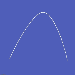
Octree technology models solids. This allows us to model the trajectory of many firings simultaneously. For the test we decided to model all trajectories within a 2 degree range in each of azimuth and elevation at a particular exit velocity (a function of the amount of propellant used). See Figure 1 for one such trajectory. NOTE: This view comes up rotating to emphasize that it's a 3-D dataset that you can control. Simply click on it to stop the rotation.
Figure 1 - Trajectory Line (1-D Element)
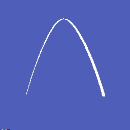
For a starting azimuth and elevation we generate a trajectory. We then do the same for an azimuth 2 degrees greater and generated the surface swept between them. See Figure 2.
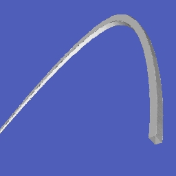
Note that all firing is from the same location (while the landings are within a spread of 2 degrees). We then do this for a 2 degree spread in elevation to form a “shell” enclosing the trajectories. See Figure 3.
The shell is then filled to form a solid. See Figure 4.

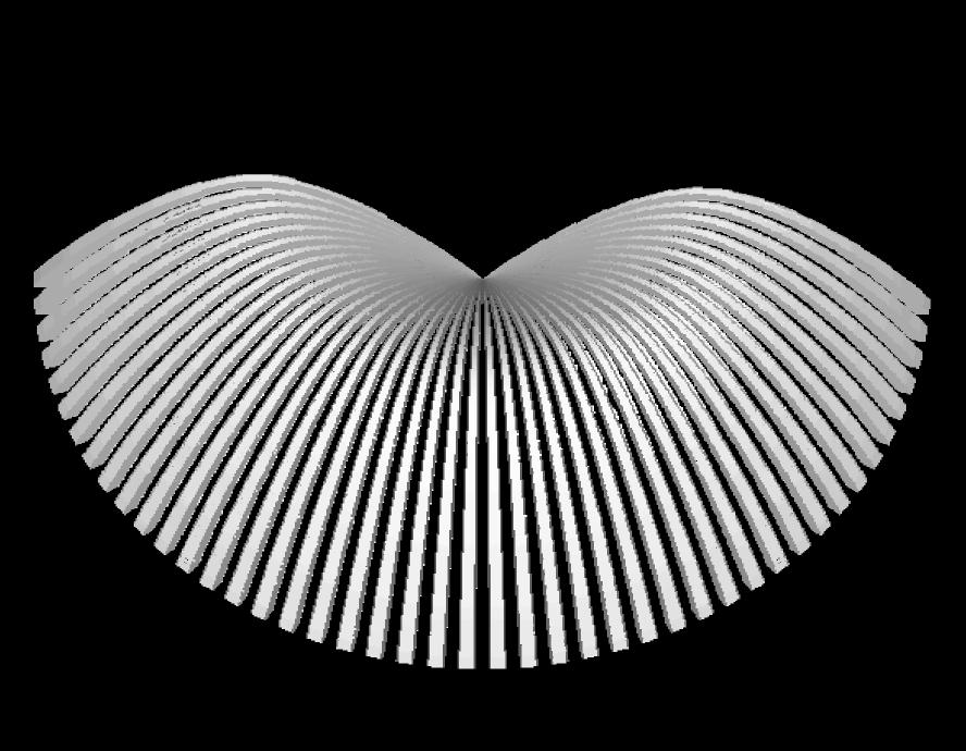
Now, of course, this is just one 2 degree by 2 degree region of our firing-direction space at one velocity. We ultimately need to fill in the remaining regions and velocities. For testing we decided to use only one velocity and to step the regions by 4 degrees in azimuth for a total of 180 degrees (45 trajectory volumes). The resulting "trajectory object" is shown in Figure 5.
If we make sure the individual trajectories volumes are disjoint (at least after they emerge from the vicinity of the firing location), we can later determine which ones end prematurely by hitting an obstacle such as a mountain. This does not necessarily mean that the individual trajectory volumes need to be separated by empty space, however. In TrueSolid ach volume element can be given a property that indicates set membership. This could be used, for example, to indicate membership in set A or set B (or both). We could thus mark this object as A, then generate the missing volumes in another object, mark it as B and then combine them to form a new object. Trajectory volumes could actually overlap (such regions would be both A and B). This could be extended to represent various power levels, forming one solid that internally represents all possible trajectories from a particular gun, at least to some specified resolution.
It is important to realize that generating this “trajectory object” can be done offline and that we have not restricted the actual paths of the trajectories (other than all trajectories within the angle ranges must stay within the trajectory volume). We can thus pre-generate this object.
It’s also important to note that within TrueSolid both the model and the later calculations are hierarchical. This means that a high resolution model (say, 0.10 or 0.01 degree increments in angle) could be calculated and saved. In the terrain intersection calculations, a low resolution version is first used. Only in regions where intersections have been found do we need to access and use the higher-resolution data. In situations with few intersections, very few calculations needed. Likewise, if there is a wall of mountains blocking most trajectories, this is also determined quickly. On the other hand, when it’s a very complex situation and it’s necessary to know the results to a high level of resolution, additional calculations are used.
Solid Terrain Map
While a region of any size could be modeled to any specified resolution, for this effort it was decided to model a 10,000 sq. km. area to a resolution of 100 m. The goal was to have a resolution high enough to be useful but low enough to be easily viewable over the Internet. A section of a terrain map was selected from a larger dataset and a satellite-generated texture map was placed on it.
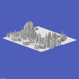
The region is shown in Figure 6. (Note: Any similarity to any real area of the world is purely coincidental.) Figure 7 shows a shaded version (no texture map).
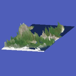
Figure 6 - Terrain Map with Texture Map
For testing we generated a solid interior. Figure 8 shows this with a “cut plain” removing a section to reveal the interior (underground regions are yellow).
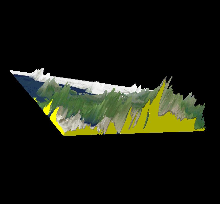
Figure 8 - Solid Terrain Map
Segmented Trajectory Solid
The first step was to place the trajectory solid in the terrain map. This is shown in Figure 9.
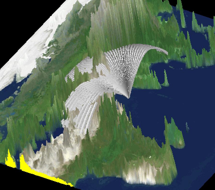
Figure 9 - Solid Terrain Map with Trajectory Object
We then did an Intersection operation between the terrain and the trajectory object. The intersected region in the trajectory volume was now made blue as shown in Figure 10.
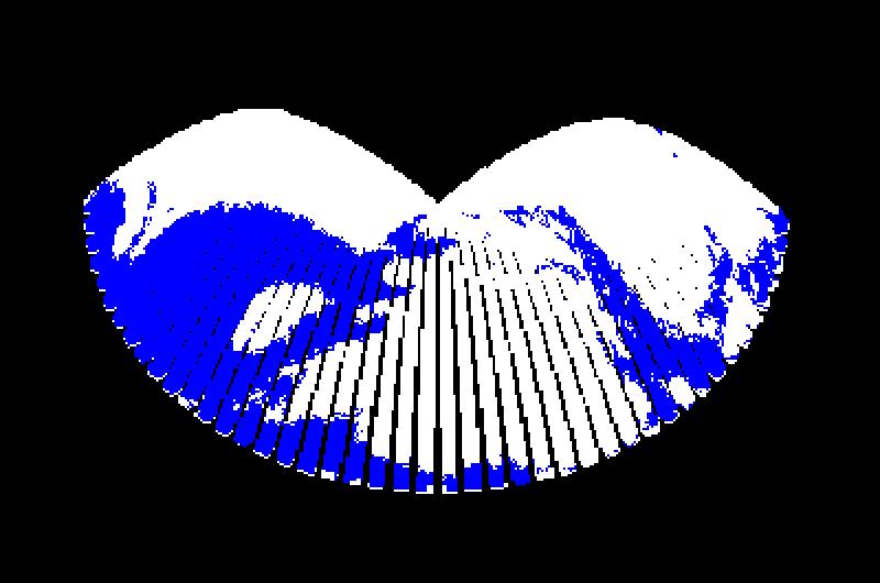
Figure 10 - Trajectory Object with Terrain Map Intersections in Blue
The next step was to perform a connectivity operation using a seed point at the trajectory origin. This volume was made red. The remaining original (white) region was now made green. It represents blocked trajectories after emerging from the terrain. The resulting object is shown in Figure 11.
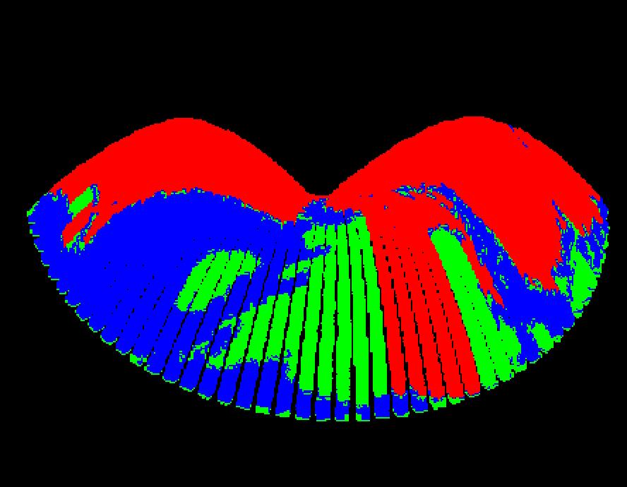
Figure 11 - Segmented Trajectory Object
Figure 12 shows it placed back in the terrain.
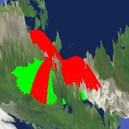
Figure 12 - Shell Map with Trajectory Object
A second test was performed using the "shell" terrain map (the underground map was removed). This results in smaller datasets (especially for transmission over the Internet) and reduced processing time. This was found to operate satisfactorily. The resulting object is shown in Figure 13.
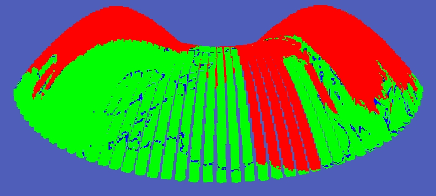
Figure 13 - Trajectory With Shell Segmentation
A second connectivity operator was performed to make intersection regions that touch red to be set to red also (blue that touches red to red). The next step was to transfer the red and green regions of the trajectory to the terrain. This was done by changing all of the regions of the surface of the terrain that intersects a red region of the trajectory object into red and the same for the region of blocked trajectories (green). The resulting shell map is shown in 14.
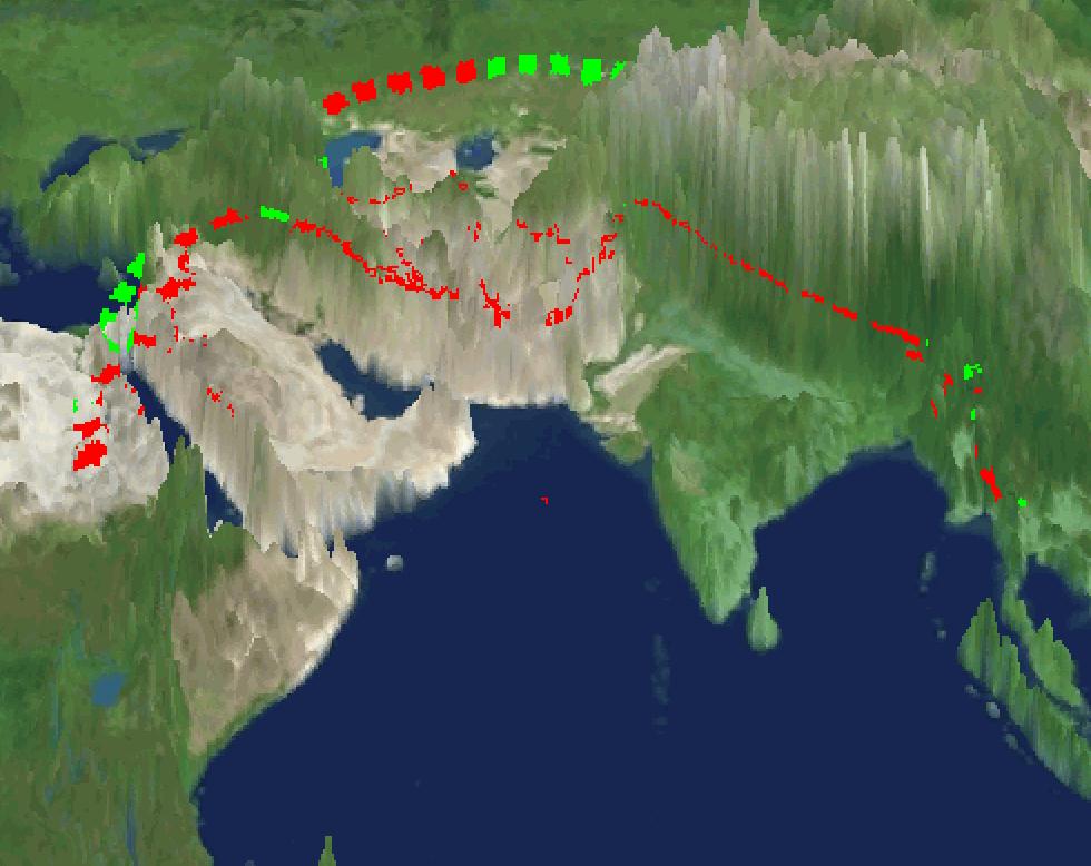
Figure 14 - Shell Map with Impact Regions
The impact regions can also be removed from the terrain for a closer examination. Figure 15 shows an example. They could be segmented into disjoint regions and analyzed independently. This could include, for example, surface area, a measure of the ruggedness of the terrain, distance to nearest road, etc. It might then be possible to do a preliminary measure of suitability for the immediate military operation.
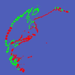
Figure 15 - Shell Map Impact Regions
Future Work
The functions implemented here could be easily reversed to find gun placements that would provide optimized coverage.
Processing Time
This effort was performed on a 1 GHz laptop computer. No graphics or other acceleration hardware was used.
Operations can be divided into two parts, those that can be pre-computed and those performed at run time. Pre-computed operations required a few seconds to a few tens-of-seconds. Run-time operations ranged from interactive (e.g., display) to a few seconds. A solution at a higher resolution would, of course, require additional time. Custom programming could make this process more efficient, however, and reduce the processing required. Also, simpler intersection situations would operate faster. Custom hardware to implement the algorithms would greatly increase the processing speed (such custom octree hardware has been developed and is in commercial use in 3-D medical computations).
Conclusions
The results of this modest effort indicate that spatial modeling and operations as implemented in the Octree TrueSolid package can be readily and effectively applied to real-world geospatial-reasoning operations of practical interest to the military and government agencies.